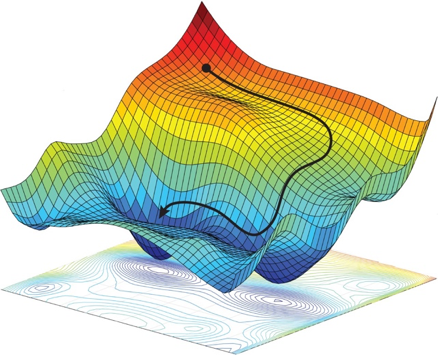
Training a Machine Learning system requires a journey through the cost terrain, where each location in the terrain represents particular values for all ML system parameters, and the height of the terrain is the cost, a mathematical value that reflects how well the ML system is performing for that parameter set (smaller cost means better performance). For a very simple ML system with only two parameters, we can visualize the cost terrain as a mountainous territory with peaks and valleys, plateaus and saddlebacks. (Deep learning cost terrains are a lot like this, only instead of three dimensions they can have millions!)
Training mathematically explores the cost terrain, taking steps in promising directions, hoping not to fall off a cliff or get lost on a plateau. Our guide in this journey is gradient descent, which calculates the best next step in the search for the best ML system parameters, which is in the lowest valley of the cost terrain.
Gradient descent can be very cautious and look at all the training samples before taking a step. This makes sure the step is a very good one, but progress is slow because it takes a long time to look at all the training samples. Or, it can make a guess and take a step after every training sample it looks at. These snap decisions make rapid steps in the cost terrain, but there is a lot of motion but little progress because each step is all about one training sample; we want the ML system to give good average performance across all the training samples.
The best way to efficiently navigate the cost terrain is a compromise between slow deliberation and snap judgement, called minibatching. This approach takes a step using a small subset of the the training set – enough to get a pretty good idea of where to go, but a small enough sample size so that the calculations can be done quickly using modern vector processors.
Read my latest iMerit blog to get a better idea of how minibatching works:
